Phase and amplitude statistics in coherent
radiation propagation.

The following work formed part of my PhD project. The work was carried out between September 2001 and May 2005 at the mathamatics department, University of Nottingham.

Supervisors: Keith Hopcraft, Eric Jakeman.
CASE sponsor: Qinetiq.

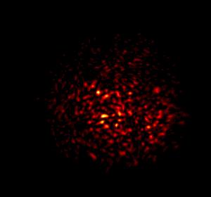
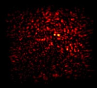
Sample beam (λ = 10^-6m) after propagation through 1km of atmospheric turbulence (C_n² = 10^-14).

What follows is a brief description of the techniques used in the computer simualtions that were performed as a part of the PhD project. Results that are presented are for the purposes of validation only, no new work or work that appears in my thesis is here. My PhD thesis ('Temporal phase and amplitude statistics in coherent radiation') is available from the British Library and the University of Nottingham.

• LIDAR systems, using lasers as remote sensors.
• Sources of noise, the Kolmogorov theory of turbulence.
• Modeling turbulence, phase screens.
• Beam propagation, the use of the Huygens-Fresnel principle to model the propagation of coherent radiation through the atmosphere.
• Statistics. Use of statistics to test the validity of the numerical technique.
• Results. A sample of the results we have obtained.
• Other work.

LIDAR systems.

Noise in atmospheric propagation.

The structure function . The correlation function . The power spectrum .

Kolmogorov developed his theory of turbulence during the early 1940s; using a model based on what he described as an energy transfer cascade he described the fluctuations in the refractive index, temperature and velocity of the atmosphere in statistical terms. He introduced inner (κI) and outer (κO) scales, derived the form of the structure function Bn(R) for the refractive index and from that the power spectrum of fluctuations φn(K). These results, along with the correlation function are very important in the field of stochastic processes for quantifying the properties of randomly fluctuating media. It is from this power spectrum that we derive our method of modelling atmospheric turbulence.

Modelling turbulence numerically.

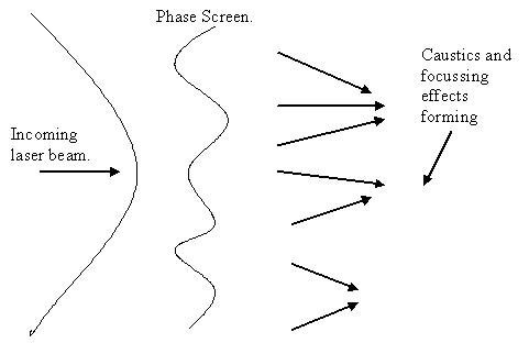
In order to model atmospheric turbulence we make use of the phase screen method. This technique was developed during the 1950s² as a way of introducing phase fluctuations into a propagating wave, one invisages a number of thin screens containing phase perturbations present at equi-distant points along the path of propagation. As you can see, (diagram right) the introduction of phase perturbations into the wave front causes fluctuations in the intensity and phase of the beam as it propagates into the space (a vacuum) beyond the screen.

The crucial question is: how do we choose the properties of the phase screen such that it accurately models the atmosphere? We employ Kolmogorov's theory of turbulence in order to produce a phase screen, we use a fast Fourier transform algorithm. We generate a sequence of random numbers which are then filtered using Kolmogorov's theory of turbulence to produce a screen with the required statistical properties, i.e. the power spectrum of these phase fluctuations is of the form φ_n(K) = 0.033C_n²k²LK^-11/3, where C_n² is the refractive index structure function, L is the propagation distance, k = 2π/λ is the wave number. This sequence of random numbers φ(x) now accurately represents a block of atmospheric turbulence. The initial laser beam, E(x,t) = A(x,t)exp(iθ(x,t)) where A is the amplitude of the beam and θ is the phase, is perturbed by the screen resulting in E(x,t) = A(x,t)exp(i(θ(x,t)+φ(x,t))). We note now that we can use as many phase screens as we like in this process, as long as they remain further apart than the outer scale of the turbulence. We can also make these screen as strong as needed by adjusting the refractive index structure parameter C_n², a value of 10^-12 is considered 'strong' turbulence while 10^-16 is 'weak'.

Beam propagation.

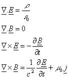With the method for numerically modelling turbulence in place, we now move on to the method of propagating our laser beam. The Maxwell's equations (right) were developed during the 19^th centuary by the legendary Scotish physicist James Clerk Maxwell, they represent possibly the most sucesful scientific theorm of all time as they accurately describe all electromagnetic fields under all conditions. Not even such revolutionary works as General Relativity or Quantum-electrodynamics have forced Maxwell's equations to be altered or adjusted. The application of these equations to our work is in the derivation that results in the wave equation.

The paraxial wave equation

The wave equation describes the motion of electromagnetic fields through any possible medium. We can simplify the standard equation somewhat by introducing assumptions based on the fact that we are looking at coherent laser beams. Assuming propagation through a vacuum (all the space between the phase screens is a vacuum) and assuming that the beam travels mostly in only the z direction (valid as the laser beam is collimated) we can reduce this to the paraxial wave equation3.

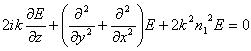
In order to use the paraxial equation, we transform it into its Fourier equivalent (see right). We can now perform our numerical experiment in the following way:

1. Set up the laser beam profile. We can use a plane wave, spherical or Gaussian beam.
2. Set up n phase screens by filtering Gaussian white noise.
3. Laser beam interacts with the first screen.
4. Fourier transform the perturbed beam and apply the paraxial wave equation.
5. Use an inverse Fourier transform to return the spectral components fo the propagated beam back into real space.
6. Repeat steps 3 to 5 for each subsequent phase screen.
7. After all phase screens have been considered, the resulting field is the initially coherent beam, now in the far field.

See the image at the top of the page for an example of a Gaussian beam after propagation through several phase screens.

Statistical measurements.

Depending on the turbulence conditions, i.e. the strength of tthe refractive index fluctuations C_n², the wavelength of the beam λ or the propagation distance L, there are several difference zones of propagation for the laser beam. The 4 images that follow are examples of laser beams from the propagation simulation used in this work, they show the different regions of propagation.

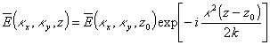
Initial beam profile. The image right shows an example of an initial beam profile. This is a Gaussian profile, such that most of the power is concentrated in the middle of the beam (lighter colours represent more intense radiation). This is what the beam looks like before proapgation through the atmosphere. We can select any beam profiile we choose and often plane or spherical beams are used in analytical calculations. The Gaussian is widely used in experiment and so it makes sense to use it here.

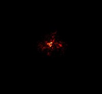
Fresnel zone. Otherwise known as the 'near-field', the Fresnel zone a region quite close to the beam emitter (in this example only 100m) where the basic shape of the initial beam profile is still intact. The statistics of the beam are very much the same as those of the initial beam, the phase statistics will be the same as those of the phase screen (as the phase of the screen was added to the collimated phase of the initial beam) as well as the intensity statistics being much the same as the initial beam. We are yet to see any of the caustics or focussing effects that were mentioned above.

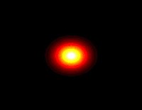
Focussing regime. This sample beam is taken at 500m from the emitter, now we begin to see some focussing effects. The ridges that are visible in the centre of the beam represent intensity levels many times larger than those present in the centre before propagation. This phenomena of concentrating power is known as focussing. It occurs quite commonly in everyday life, think of the patterns one sees on the bottom of a swimming pool due to the lights shining above. That is due to the water acting as a turbulent medium and causing focussing effects, much in the same way that the atmosphere causes a laser beam to focus. It is here that the statistics of the beam begin to change, the intensity can now be described by log-normal statistics4, although this is at best an approximation. No-one has yet been able to fully describe the properties of a field in the focussing regime analytically.

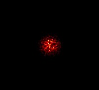
Fraunhofer zone. This final image shows the far field regime, or the Fraunhofer zone. Here is is obvious that the beam has spread and diverged as a result of the interaction with turbulence. We get a Gaussian speckle pattern5, such that the intensity statistics are described by a negative exponential distribution and the phase derivative is described by a student-t5 distribution. The image here shows the same beam as used above, this time we have allowed it to propagate to 1.5km.

It is clear from the descriptions given of each of the zones that we define the properties of the laser beam in statistical terms. It has already been made clear that a deterministic approach is unfeasable for a physical situation when we are dealing with the atmosphere (whose characteristics constitute a random process) and so this stochastic modelling and statistical data processing is essential. Statistical measures that can be used are:

Scintillation index <I2>/<I>2

This is the second moment of the intensity I (fourth moment of the amplitude) normalised against the mean-intensity squared, it tells us a lot about the region into which the beam has propagated. Many studies have been made about the behaviour of the scintillation index under various turbulence conditions and using various beam profiles6, 7, 8.

Intensity Spectrum SI(ω)

The intensity spectrum is simply the Fourier transform of the intensity data, it is defined in terms of a frequency space variable (here we use ω). It gives us information about the spectral components of the intensity in the beam. Several theoretical studies exist that describe the behaviour of SI(ω) in certain turbulence regimes. These studies have been validated (and in some circumstances challenged) by groups using numerical simulations similar to the ones described here9, 10.

Intensity-Weighted phase derivative J

This statistic is defined as the product of the intensity and the phase derivative, I(dφ/dt). The phase derivative is a very important statistic in LIDAR systems as it allows us to look directly at the perturbed phase of the returning beam. We cannot look directly at the phase derivative itself as its fluctuations are too rapid for any statistical measure to converge. It was proposed11 that one weight the phase derivative with the intensity as large changes in phase are often associated with small intensity values. Thus a statistical measure of J give us an insight into the behaviour of dφ/dt.

Phase power spectrum Sφ(ω)

The phase power spectrum is the Fourier transform of the phase data, thus it is defined similarly to the intensity spectrum above. Sφ(ω) is linked to the power spectrum of the turbulent layer through which the beam propagates (See 'Noise' above) in that they both describe the spectral components of the phase present in the beam. Thus Sφ(ω) can be used experimentaly to investigate the properties of the real atmosphere, we can use the phase power spectrum to directly compare numerical simulation to experimental data. The properties of Sφ(ω) were investigated for plane and spherical waves under weak turbulence conditions by Clifford12.

Results.

What follows now is some results that we have obtained using our numerical 'experiments'. The purpose of these results is as a benchmark for more complicated simulations. Results presented here are compared to analytical derivations, by doing this we hope to ensure that our technique is sound before moving into areas that do not yield to analysis.

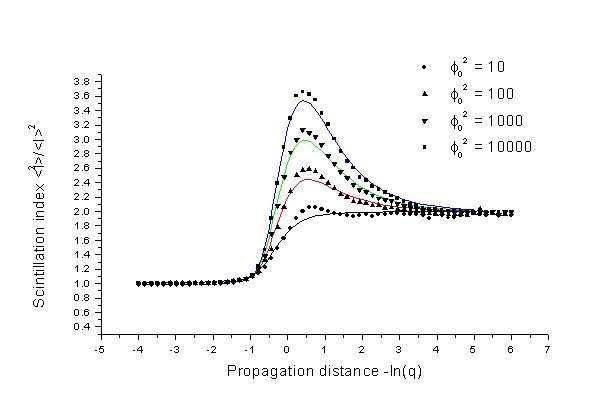
The plot (right) of the scintillation index of a plane wave propagating through various levels of strong turbulence shows good correlation between simulation (symbols) and theory (solid lines). The theory which we are using for comparison is the work of Jakeman and McWhirter7. The strength of the turbulence is characterised by the mean square phase shift imparted on to the beam by the screen, only a single screen is used in each of these propagation problems. The distance parameter (here -ln(q)) is a dimensionless variable normalised by the wavelength, strength and correlation properties of the screen. We note that at long distances (-ln(q) = 5) the scintillation index approaches a value of 2; this is consistant with the idea that the beam converges to Gaussian statistics at long propagation distances and under strong turbulence conditions.

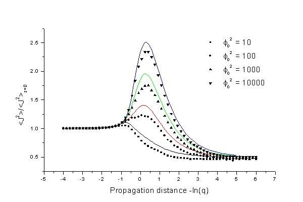
The plot shown on the left here is a measure of the second moment of the intensity-weighted phase derivative J. Notice that the the distance range over which the statistic changes is similar to that over which the scintillation index above evolves. The second moment of the J statistic is normalised by its value at the phase screen. This is because the odd order moments of J are all zero (this is easily shown) and so the statistic cannot be normalised in the same way as the scintillation index. Once more we compare simulations (symbols) with theory11 (solid lines) and note a good match. The two sets of results displayed here indicate that our simulation technique is valid and corroborates theoretical results.

Further / other areas of work.

There are several other methods available to us in terms of validatiing the simulation technique; theortical results exist that refer to the spreading of Gaussian beam profiles in 2 dimensions, scintillation indicies for weak turbulence as well as spectra for both the intensity and phase in spacial and temporal terms.

We note also that in the two plots given in the above section were both obtained using a simplified spectrum to filter the phase screen data. We made use of a Gaussian filter (φ_n(ω)) ~ exp(-ω²/ξ²)) which yields more easily to analysis. An area of research is to look at several difference turbulence models (each of which will be based loosely on the Kolmogorov theory of turbulence) and compare numerical simulation with experiment. The objective being to find the model that most accurately describes atmospheric turbulence.

The ultimate application of our work is in the design and improvement of LIDAR systems for use in the field of vibrometry. To this end we believe that the most important area of research is in the phase power spectrum. It is this statistic that is used in laser vibrometry systems to detect frequency alterations in the retro-reflected beam, thus it is the behaviour of this statistic under various turbulence conditions that we will concentrate on in the thesis to this PhD project.

References.

1. O Svelto, 'Principles of Lasers', 3rd Ed, (Plenum Press, 1993).
2. H.G.Booker, T.A.Ratcliffe and D.H.Schinn, 'Diffraction from an irregular screen with applications to ionospheric problems', Phil.Trans.Roy.Soc. A, 242, 579-609, (1950).
3. L. C. Andrews, R. L. Phillips, 'Laser Beam Propagation through Random Media.' (SPIE 1998).
4. E. Jakeman, P. N. Pusey, 'A model for Non-Rayleigh Sea Echo.' IEEE trans. on antennas and propagation, AP-24, 806-814, (November 1976).
5. J. W. Goodman, 'Statistical Optics', (Wiley-Interscience 1985).
6. R.P.Mercier, 'Diffraction by a screen causing large random phase fluctuations', Proc. Camb.Phil.Soc. A 58, 382-400, (1962).
7. E. Jakeman, J.G. McWhirter, 'Correlation function dependence of the scintillation behind a deep random phase screen', J. Phys, A: Math. Gen. 10, 1599-1643, (1977).
8. E. N. Bramley, 'Diffraction of an angular spectrum of waves by a phase-changing screen.' J. Atmos. Terr. Phys., 29, 1-28, (1966).
9. J. M. Martin, S. M. Flatte, 'Intensity images and statistics from numerical simulation of wave propagation in 3-D random media.', Applied Optics, 72, 2111-2126, (1998).
10. J. M. Martin, S. M. Flatte, 'Simulation of point-source scintillation through three-dimensional random media.', J. Opt. Soc. Am., A 7, 838-847 (1990).
11. E. Jakeman, S. M. Watson, K. D. Ridley, 'Intensity- weighted phase-derivative statistics.', J. Opt. Soc. Am, 18, 2121-2131, (Sept 2001).
12. S. F. Clifford, 'Temporal-Frequency Spectra for a Spherical Wave Propagating through Atmospheric Turbulence.' J. Opt. Soc. Am., 61, 1285-1292, (October 1971)